Semantic segmentation
Semantic Segmentation Services
Batch inference with established segmentation models for street scenes, remote sensing, medical imaging and industrial inspection — turning your existing image dataset into masks, measurements and review-ready outputs.
Overview
A mask is only useful if you can count something with it
Semantic segmentation assigns every pixel in an image to a class: road, building, vegetation, sky, defect, tissue, crop. What makes it worth doing is the step after that. A mask on its own is a picture; the deliverable is the table it produces — how much of this image is vegetation, how large is this defect in millimetres, how many hectares of this field are under one crop, how did all of that change between two dates.
This is an inference service, not a model-development engagement. We select an established public or client-supplied checkpoint whose existing class system matches the question, standardise your files, run it at scale, post-process the output and package the results. We do not annotate a new training set, train a model from scratch or fine-tune one to create unsupported classes.
That boundary matters: a Cityscapes checkpoint cannot become a crack detector simply because both tasks are called segmentation. Before a full run, we test representative samples for domain fit, resolution, class coverage and output quality. If no mature checkpoint supports the requested classes reliably, we say so rather than hiding a training project inside an inference quote.
Four service areas
What we run in each field, and what the output looks like
Four domains that share a pipeline shape and almost nothing else. Each is covered in full before the next begins: the checkpoints available, the workloads they suit, a sample of real output, the accuracy their authors published, and the class systems those figures were measured on. Dataset names describe what a checkpoint already knows — not something we retrain per project.
Street-scene segmentation
Models
SegFormer, DeepLabv3+, Mask2Former, OneFormer, HRNet, BiSeNet and PP-LiteSeg checkpoints. We choose between accuracy, small-object boundary quality and throughput; semantic, instance or panoptic output is selected according to whether the result needs area, count or both.
Datasets and class systems
Cityscapes (19 road-scene classes), Mapillary Vistas (66 globally varied street classes), ADE20K (150 scene-parsing classes), BDD100K and IDD. The selected checkpoint's native labels determine what can be reported; we do not add new labels during the project.
Suitable workloads
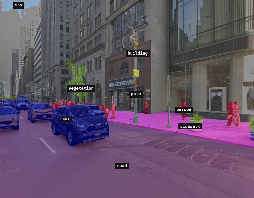
Google or Baidu street-view frames, 360 panoramas, Mapillary or KartaView imagery, dashcam video and fixed-heading photographs. Typical outputs include green-view and sky-view share, road and sidewalk coverage, frontage composition, vehicle/person pixels and network-level aggregates.
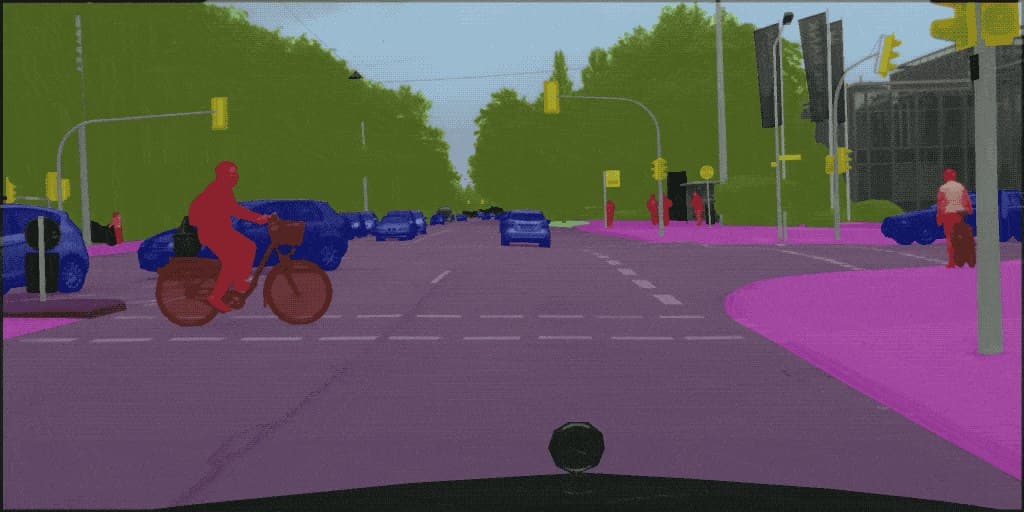
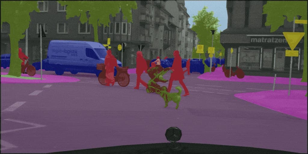
Sample output · street and driving scenes
Road, sidewalk, building, vegetation, sky, vehicles and people separated under a Cityscapes-style class system. This is the output shape behind green-view share, sky openness, frontage composition and mobility indicators.
Published accuracy and class system
Cityscapes is the reference benchmark for 19-class road scenes; ADE20K is the wider 150-class scene-parsing set used when a project needs street furniture, awnings, signage or building detail beyond the Cityscapes vocabulary. The same architecture scores far lower on ADE20K — not because it degrades, but because 150 classes is a harder question than 19.
Cityscapes val · mIoU
- SegFormer-B51024² · NeurIPS'2184.0
- OneFormerSwin-L · s.s.83.0
- Mask2FormerSwin-L · s.s.82.9
- HRNetV2-W481024×204881.1
- DeepLabv3+Xception-6578.8
- PP-LiteSeg-B2STDC2 · 102.6 FPS78.2
- SegFormer-B03.8M · 15.2 FPS76.2
- BiSeNetV2512×1024 · 156 FPS73.4
ADE20K val · mIoU
- OneFormerSwin-L · s.s.57.0
- Mask2FormerSwin-L · s.s.56.1
- UPerNet + Swin-Ls.s. · ms+flip 53.552.1
- SegFormer-B5640²51.8
- SegFormer-B03.8M params37.4
| Dataset | Classes | What the classes cover |
|---|---|---|
| Cityscapes | 19 | Grouped by the authors into 7 categories: flat (road, sidewalk); construction (building, wall, fence); object (pole, traffic light, traffic sign); nature (vegetation, terrain); sky; human (person, rider); vehicle (car, truck, bus, train, motorcycle, bicycle). |
| Mapillary Vistas | 66 (v1.2) · 124 (v2.0) | Seven top-level groups: animal, construction, human, marking, nature, object and void. Adds street detail Cityscapes has no label for — lane markings, kerbs, manholes, benches, bins, street lights — across imagery from six continents. |
| ADE20K | 150 | Scene parsing across indoor and outdoor imagery: background classes (wall, sky, floor, road, water, mountain, grass) mixed with discrete objects (car, person, tree, signboard, awning, stairs, railing, streetlight). |
| BDD100K | 19 | Semantic labels aligned with the Cityscapes 19; the imagery is US dashcam footage with much wider spread of weather, time of day and road type. |
| IDD | 26 (common level) | A four-level hierarchy that can be read at 7, 16 or 26 classes; adds South Asian road elements such as auto-rickshaws, road barriers, billboards and unsurfaced drivable shoulder. |
| COCO-Stuff | 171 | 80 object classes plus 91 stuff classes — used when the imagery is general photography rather than a road scene. |
Remote-sensing segmentation
Models
U-Net and U-Net++, DeepLabv3+, SegFormer, UPerNet with Swin or ConvNeXt, HRNet and specialised GeoSeg checkpoints. Large rasters are tiled with overlap, inferred in batches, edge-blended and reconstructed without losing georeferencing.
Datasets and class systems
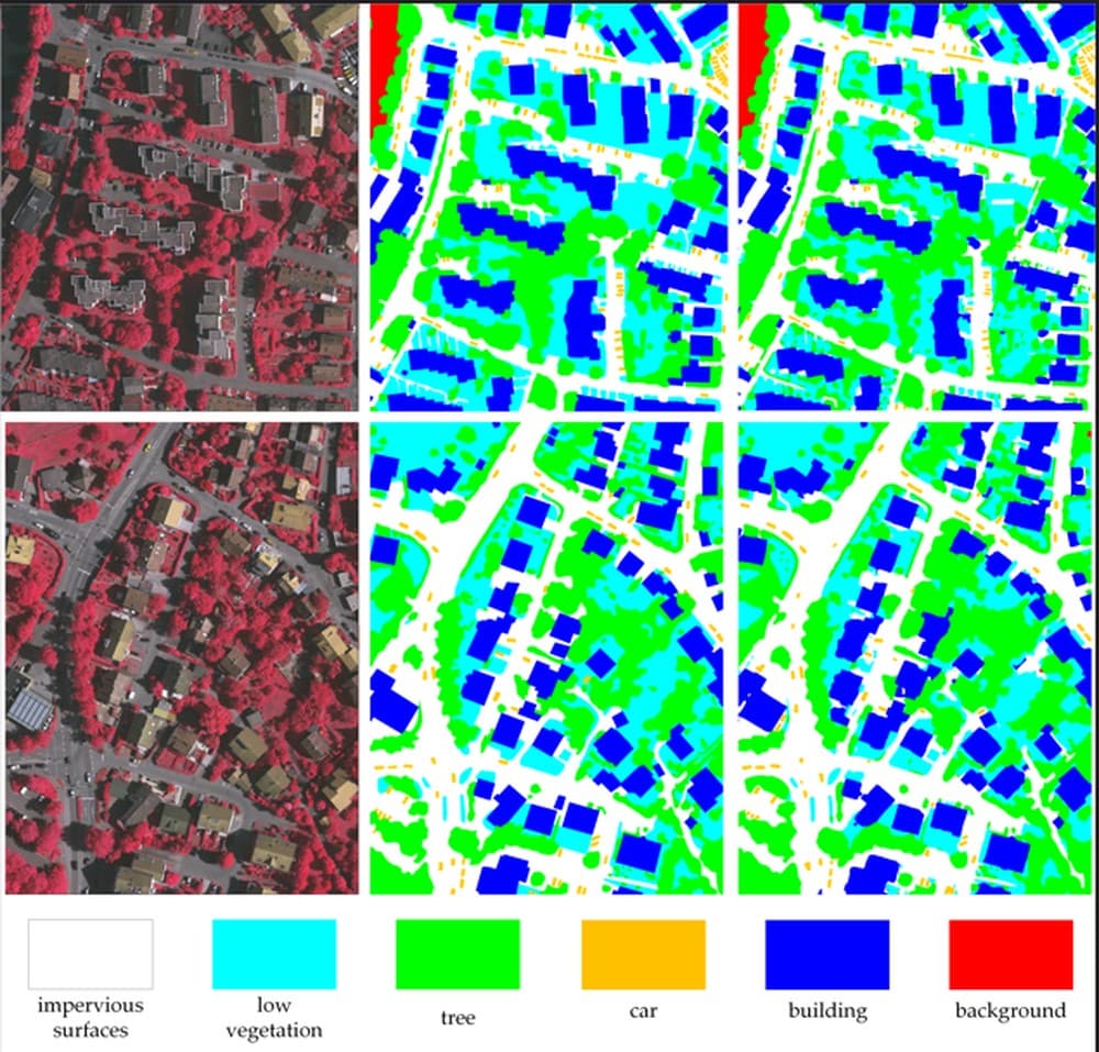
LoveDA for urban/rural land cover; ISPRS Potsdam and Vaihingen for impervious surface, building, vegetation, tree and car; DeepGlobe and DynamicEarthNet for land-cover mapping; SpaceNet for buildings and roads. Sensor, ground sampling distance and band configuration must match the checkpoint.
Suitable workloads
Satellite, aerial and drone orthophotos for land-cover area, building footprints, road extraction, vegetation/canopy coverage, impervious surface, parcel summaries and time-series change. Outputs can remain raster or be vectorised to polygons and lines for GIS.
Sample output · aerial and satellite imagery
Land-cover classes extracted from a georeferenced tile and rebuilt into a seamless mask. Area, building footprints and vegetation coverage are computed from this, per parcel or per date.
Published accuracy and class system
Land-cover scores sit far below street-scene scores, and that is normal: classes such as barren and forest are genuinely ambiguous at 0.3 m ground sampling distance, and the LoveDA benchmark deliberately mixes urban and rural domains. Where imagery matches the benchmark closely — ISPRS aerial tiles at 5–9 cm — the same architectures score in the mid-eighties.
LoveDA test · mIoU
- UNetFormerResNet-18 · GeoSeg52.4
- HRNetW3249.8
- FactSegResNet-5048.9
- PSPNetResNet-5048.3
- UNet++ResNet-5048.2
- UNetResNet-5047.8
- DeepLabv3+ResNet-5047.6
- FCN-8sVGG-1646.7
ISPRS Potsdam / Vaihingen · mIoU
- FT-UNetFormer · PotsdamSwin-B87.5
- UNetFormer · PotsdamResNet-1886.5
- FT-UNetFormer · VaihingenSwin-B84.0
- UNetFormer · VaihingenResNet-1882.5
| Dataset | Classes | What the classes cover |
|---|---|---|
| LoveDA | 7 | Background, building, road, water, barren, forest, agriculture. 0.3 m GSD over three cities, split into an urban and a rural domain to test transfer. |
| ISPRS Potsdam / Vaihingen | 6 | Impervious surface, building, low vegetation, tree, car, clutter/background. True orthophotos at 5 cm (Potsdam) and 9 cm (Vaihingen), with DSM available. |
| DeepGlobe Land Cover | 7 | Urban, agriculture, rangeland, forest, water, barren, unknown — satellite imagery at 0.5 m, aimed at country-scale mapping. |
| DynamicEarthNet | 7 | Impervious surface, agriculture, forest and other vegetation, wetlands, soil, water, snow and ice — daily time series, built for land-cover change rather than a single date. |
| SpaceNet | Buildings / roads | Building footprint polygons and road centreline networks, released city by city; the target is a vector layer, not a land-cover raster. |
| UAVid | 8 | Building, road, static car, moving car, tree, low vegetation, human, background clutter — oblique drone video, closer to street level than to nadir imagery. |
Medical-image segmentation
Models
nnU-Net task checkpoints, U-Net variants, UNETR and Swin UNETR for volumetric data, plus MedSAM or SAM-Med2D for prompt-assisted masks. We preserve spacing, orientation and slice order, and can return both per-slice masks and reconstructed 3D volumes.
Datasets and target anatomy
Medical Segmentation Decathlon and BTCV for multi-organ CT, BraTS for brain tumours, KiTS for kidney and renal tumour, LiTS for liver and tumour, plus organ-specific public checkpoints. A checkpoint is used only for the modality, anatomy and acquisition range it was built to support.
Suitable workloads and boundary
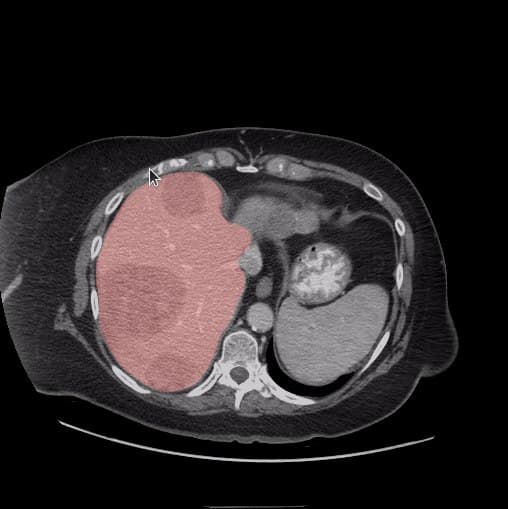
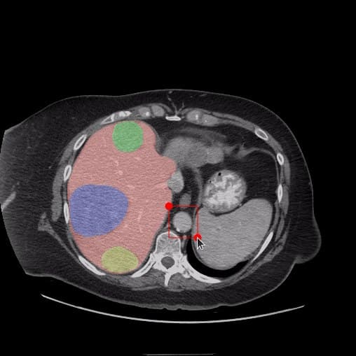
Batch processing of de-identified CT, MRI, ultrasound or endoscopy datasets for research, teaching and retrospective measurement: organ volume, lesion region, boundary and longitudinal comparison. Outputs are not presented as a diagnosis or a clinically certified medical device result.
Sample output · medical imaging
Supported organs and regions of interest delineated on CT slices with voxel geometry preserved, so volume and boundary can be measured. Research and measurement processing, not diagnosis.
Published accuracy and class system
Reported as Dice rather than IoU. The headline average hides the part that matters for measurement work: large organs are close to solved, while small or low-contrast structures are several points behind, and that gap widens on scanners and protocols the checkpoint has not seen.
BTCV abdominal CT · average Dice
- Swin UNETRCVPR'2291.8
- UNETRCVPR'2289.1
- nnU-Net3D full-res88.8
- PaNN85.4
- CoTr84.4
- TransUNet83.8
- SETR-PUP79.7
Swin UNETR · Dice per organ
- Liver98.5
- Spleen97.6
- Right kidney95.8
- Left kidney95.6
- Stomach95.3
- Aorta94.8
- Inferior vena cava90.4
- Portal & splenic veins89.9
- Pancreas89.7
- Gallbladder89.3
- Esophagus87.5
- Adrenal glands84.6
| Dataset | Targets | What the labels cover |
|---|---|---|
| BTCV | 13 organs | Spleen, right and left kidney, gallbladder, esophagus, liver, stomach, aorta, inferior vena cava, portal and splenic veins, pancreas, right and left adrenal gland — contrast abdominal CT. |
| Medical Segmentation Decathlon | 10 tasks | Brain tumour, heart, liver and tumour, hippocampus, prostate, lung nodule, pancreas and tumour, hepatic vessel and tumour, spleen, colon cancer — across CT and multi-sequence MRI. |
| BraTS | 3 sub-regions | Whole tumour, tumour core, enhancing tumour, derived from four co-registered MRI sequences (T1, T1ce, T2, FLAIR). |
| KiTS | 2–3 classes | Kidney and renal tumour; KiTS21 onward adds renal cyst as a separate class. |
| LiTS | 2 classes | Liver and liver tumour on contrast-enhanced CT, with highly variable lesion size. |
| AMOS | 15 organs | Abdominal multi-organ across both CT and MRI, from multiple centres and scanners — the closest public proxy for mixed-source clinical archives. |
Industrial segmentation
Models
Anomalib implementations of PatchCore, PaDiM, EfficientAD, FastFlow and Reverse Distillation for anomaly localisation, plus mature U-Net, DeepLabv3+ or SegFormer checkpoints where a known defect class already has a public or client-supplied model.
Datasets and defect types
MVTec AD, VisA, BTAD and KolektorSDD cover surfaces and products such as metal, fabric, tile, cable, capsule, bottle, transistor and printed circuit boards. They support anomaly heat maps and masks for scratches, cracks, contamination, missing parts and surface irregularities.
Suitable workloads and boundary
Repeatable inspection imagery with stable camera position, lighting, scale and product appearance. We can measure defect area, length, shape and pass/fail thresholds from a suitable checkpoint; highly variable production scenes or novel defect categories usually require model development and are outside this service.
Sample output · industrial surfaces and defects
Input, ground truth, predicted heat map, predicted mask and final result for one defect. The mask is what makes defect area, length and tolerance measurable rather than merely visible.

Published accuracy and class system
Anomaly detection is scored as AUROC rather than mIoU, and the image-level figures are all above 97.9 — which means they no longer separate methods usefully. Pixel-level AUROC and the PRO metric are the numbers that predict whether a heat map is tight enough to measure a defect from, so we quote both.
MVTec AD · image-level AUROC
- PatchCoreensemble · CVPR'2299.6
- RD++CVPR'2399.4
- FastFlowWR5099.4
- EfficientAD-MWACV'2499.1
- EfficientAD-SWACV'2498.8
- Reverse DistillationWR5098.5
- PaDiMEfficientNet-B597.9
MVTec AD · pixel-level AUROC
- FastFlowWR5098.5
- RD++PRO 95.098.3
- PatchCorePRO 93.598.1
- Reverse DistillationPRO 93.997.8
- PaDiMPRO 92.197.5
| Dataset | Categories | What the data covers |
|---|---|---|
| MVTec AD | 15 categories · 73 defect types | Five textures (carpet, grid, leather, tile, wood) and ten objects (bottle, cable, capsule, hazelnut, metal nut, pill, screw, toothbrush, transistor, zipper); 5,354 images, defects annotated at pixel level. |
| VisA | 12 objects | PCB1–4, capsules, cashew, chewing gum, fryum, macaroni1–2, candle, pipe fryum; 10,821 images (9,621 normal, 1,200 anomalous), including multi-instance scenes. |
| MVTec LOCO | 5 categories | Breakfast box, juice bottle, pushpins, screw bag, splicing connectors — covers logical anomalies (wrong count, wrong part, misplacement) as well as structural ones. |
| BTAD | 3 products | 2,540 images of real production parts; surface and shape defects photographed on the line rather than in a lab. |
| KolektorSDD / SDD2 | Surface cracks | Electrical commutators and production-line surfaces with pixel-level crack annotation — the closest public analogue to a fixed-fixture inspection station. |
Every figure above is taken from the official paper or model zoo of the method named, not from our own evaluation. Backbones, input resolution and single- versus multi-scale testing differ between rows, and each chart uses a truncated axis stated in its caption — so read them as orders of magnitude, not as a ranking to a tenth of a point. What a checkpoint scores on its own benchmark is also an upper bound: on your imagery, with your classes, the number will be lower. That is why every engagement starts with a pilot run on your samples, whose measured result is what we quote against. Sources: SegFormer (NeurIPS 2021), DeepLab model zoo, HRNet, Mask2Former (CVPR 2022), OneFormer, PP-LiteSeg / PaddleSeg, Swin Transformer, LoveDA (NeurIPS 2021 D&B), GeoSeg, Swin UNETR (CVPR 2022), PatchCore (CVPR 2022), FastFlow, EfficientAD (WACV 2024), RD++ (CVPR 2023), PaDiM.
Demonstration imagery from open-source projects, used under their licences: MMSegmentation and Anomalib (Apache-2.0), MedSAM (Apache-2.0) and GeoSeg (GPL-3.0). Shown to illustrate what each class of output looks like; project work is run on your imagery.
Scope
What you receive
Masks are the intermediate product. The statistics derived from them, and the evidence that they are trustworthy, are the deliverable.
Per-image masks
Indexed PNG or single-band GeoTIFF, one value per class, at the resolution of the source image.
Class colour map
The palette and its class mapping as data, so masks render identically wherever they are opened.
Per-class statistics
Pixel count, area and share per class per image, in real units where the imagery is georeferenced or calibrated.
Vector polygons
Masks converted to simplified polygons with a tolerance you choose, for GIS and CAD workflows.
Object instances
Where the question is 'how many' rather than 'how much', connected regions counted and measured individually.
Confidence layer
Per-pixel confidence written alongside the mask, so low-certainty regions can be reviewed rather than trusted blindly.
Accuracy report
Overall and per-class IoU, precision and recall against a manually scored sample, with the sample included.
Change comparison
Where two dates exist, per-class gain and loss between them, with the pairing method stated.
Method record
Checkpoint name and licence, native class map, input transformation, inference settings, thresholds and post-processing, written down and versioned.
Processing manifest
One record per input file with processing status, output path, warnings and failures, so large runs can be audited and resumed.
Output formats
Delivered the way your stack expects
- PNG / TIFF masks
- Indexed masks plus optional colour-rendered overlays for review and reporting.
- GeoTIFF
- Georeferenced masks aligned to the source imagery, ready for QGIS and ArcGIS.
- GeoJSON / Shapefile
- Vectorised classes with per-polygon area and class attributes.
- NIfTI / DICOM-derived masks
- Slice-aligned or reconstructed volumetric masks for medical research workflows, with source identifiers preserved.
- CSV / Excel
- Per-image and aggregated class statistics with the accuracy report as a separate sheet.
- JSON manifest
- Input-to-output mapping, model version, class schema, processing status and exception notes for every file.
Use cases
What clients use it for
- Streetscape indicatorsTurn street-level imagery into greenery, enclosure and frontage measures across a whole network.
- Land cover and land useClassify aerial or satellite tiles into surface types, then measure area and change between dates.
- Crop and vegetation mappingSeparate crop types, canopy and bare soil from drone or satellite imagery, reported by parcel.
- Medical image analysisSegment organs, lesions and regions of interest for research and teaching datasets.
- Batch dataset processingRun a compatible mature checkpoint over an existing image collection and return standardised masks, measurements and exceptions.
Sample dataset
What you actually receive
Sample project data. Small, thin classes such as people and poles always score lower than large contiguous ones; reporting them separately is the point, because an averaged figure hides exactly the classes most likely to be wrong.
| Class | Pixel share % | IoU | Precision | Recall | Samples |
|---|---|---|---|---|---|
| Road surface | 31.4 | 0.94 | 0.96 | 0.97 | 480 |
| Building | 24.8 | 0.91 | 0.93 | 0.95 | 480 |
| Vegetation | 18.2 | 0.89 | 0.92 | 0.94 | 480 |
| Sky | 12.6 | 0.97 | 0.98 | 0.99 | 480 |
| Vehicle | 7.1 | 0.83 | 0.88 | 0.90 | 480 |
| Person | 1.4 | 0.68 | 0.79 | 0.76 | 480 |
How it works
Five steps, every project
- Step 01
Send representative samples
We inspect imagery type, resolution, bands or medical modality, required classes, volume and the measurement the result must support.
- Step 02
We check checkpoint fit
We match the request to mature public or client-supplied models and confirm that the existing class map covers the requested output.
- Step 03
We run a pilot batch
A representative subset is inferred and reviewed first. If domain fit is poor or training would be required, we stop and say so before a full run.
- Step 04
We process the full dataset
Files are standardised, batched through the fixed checkpoint, post-processed and recorded in a resumable processing manifest.
- Step 05
We validate and deliver
We check a sample and deliver masks, statistics, vectors or volumes, confidence and exception records, and the complete method note.
Projects are priced on file count and size, imagery type, preprocessing and tiling requirements, selected mature checkpoint, output formats and validation depth. Training, fine-tuning and new-class annotation are not included. Send representative samples and the required classes, and we first confirm model fit before issuing a fixed inference quote.
FAQ
Questions we get asked
What is semantic segmentation?
It is the assignment of every pixel in an image to a class, as opposed to classification, which labels the whole image, and detection, which draws a box around an object. Segmentation is the right tool when the answer is an area or a shape — how much of this scene is vegetation, what is the extent of this defect — rather than a yes or no.
What imagery can you work with?
Street-level and 360 panoramas, drone and aerial photography, satellite tiles, industrial inspection images, video frames, and medical imaging such as CT, MRI, ultrasound and endoscopy. The practical constraints are resolution relative to the smallest class you care about, and whether the classes are actually visible in the imagery you have.
Do you train or fine-tune a model for us?
No. This service runs established pre-trained or client-supplied checkpoints over your dataset. It does not include collecting annotations, training from scratch or fine-tuning for new classes. You usually do not need labelled training data, but the classes and imagery domain must already be supported by a mature checkpoint. We verify that with representative samples before quoting the full run.
How accurate is it?
It depends on the class, which is why we report per class rather than as one headline number. Large contiguous classes such as road, building and sky typically reach 0.90 or better IoU; small or thin classes such as people, poles and wires sit lower. Every project is validated against a hand-scored sample, and that sample is delivered with the results so you can audit the claim.
What if no existing model fits our data?
Then we do not pretend that batch inference will solve it. We explain the mismatch — unsupported classes, sensor or modality shift, resolution, acquisition conditions or licence — and recommend a separate model-development route. Training work is outside this service.
Can you process video rather than stills?
Yes. Video is sampled to frames at an interval that suits the question, segmented frame by frame, and optionally smoothed across time so a class does not flicker between adjacent frames. Results can be reported per frame, per second or aggregated across a whole clip.
More services
Often combined with
Street View Data
Large-scale street view imagery collection, processing and structured dataset delivery.
Learn MorePOI Data
Business and point-of-interest records with categories, coordinates and attributes.
Learn MoreGoogle Maps Data
Structured business listings with coordinates, categories, ratings and opening hours.
Learn MoreKeep exploring
Where to go next
Related services
- Street View DataLarge-scale street view imagery collection, processing and structured dataset delivery.
- GIS AnalysisSpatial analysis and geographic data processing, from overlays to network models.
- Geospatial DataLocation, road, boundary and land-use datasets, cleaned and projected correctly.
- Data CollectionCustom data collection and structured datasets built around one specific question.
Related reading
- Street View Data Processing with Semantic SegmentationCollection is only the first stage. A large street view image set becomes usable data when headings, classes, seasonality and validation are controlled across the whole pipeline.
- Planning Large-Scale Google Street View CollectionBefore collecting thousands of images, use free metadata requests to measure coverage, image age and expected volume across the whole sampling frame.
Next step
Have a specific data requirement?
Tell us the geography, the fields and the cadence you need for semantic segmentation. You get a scoped plan, a sample and a fixed price before any work starts.