Street View Data Processing: From Semantic Segmentation to Defensible Metrics
Collection is only the first stage. A large street view image set becomes usable data when headings, classes, seasonality and validation are controlled across the whole pipeline.
- Author
- HuiTu Technology
- Published
- Updated
Running a segmentation model over street-level imagery is the easy part. Open urban-scene models are good, they run fast, and the coloured output looks convincing enough that people accept whatever percentages come out the other side.
The hard part is everything between the pixel map and a number someone will act on. This is a walk through the decisions that sit in that gap, in the order they actually bite.
One point, four headings, one profile
A single camera direction is not a measurement of a street; it is a measurement of what the camera happened to face. Point the camera at a park and the street looks green. Point it down the carriageway and the same location looks barren.
- Render four perspective crops per sample point at 0°, 90°, 180° and 270°, compute indicators per crop, then average to one profile per point.
- Keep the field of view fixed across the whole project. Widening it pulls in more sky and more building tops, which shifts every share you are about to compute.
- Keep pitch fixed too, and near horizontal. A slight upward tilt is the fastest way to inflate a sky share without anyone noticing.
- Reproject from the panorama to flat perspective crops before inference. Models are trained on ordinary rectilinear photographs, and feeding them equirectangular imagery puts curved buildings and stretched skies in front of a network that has never seen either.
- Keep the per-heading values alongside the averaged profile. Their spread tells you whether a point sits on a genuinely uniform street or on a boundary between two very different ones.
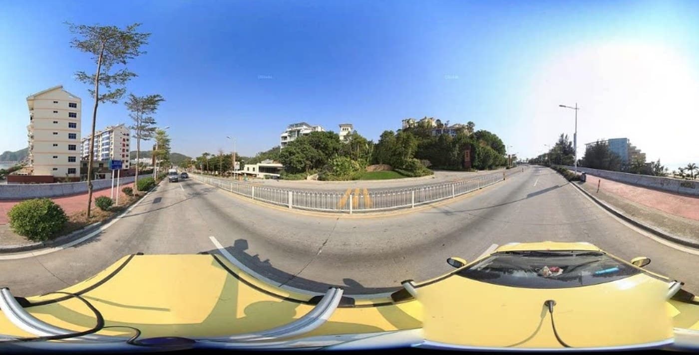
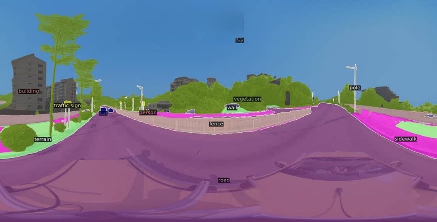
Defining the indicators precisely
Each indicator below is a share of classified pixels, which makes the class definitions load-bearing. Write the definition down next to the number, because two teams computing a green view index will disagree by several points purely on which classes they counted.
| Indicator | Definition | Most sensitive to |
|---|---|---|
| Green view index | Vegetation pixels as a share of the visible frame, averaged across headings | Capture month, and whether grass and terrain are counted as vegetation |
| Sky share | Sky pixels as a share of the frame | Camera pitch, field of view, and overexposure on bright days |
| Enclosure proxy | Vertical surface — building, wall, fence — against visible sky | Tree canopy, which occludes facades and lowers the ratio in summer |
| Ground composition | Road, sidewalk and terrain shares | Parked vehicles occluding the carriageway and the kerb |
| Pedestrian and vehicle presence | Detected counts, reported next to pixel shares | Time of day and day of week, which are not controllable in platform imagery |
import numpy as np

# Cityscapes evaluation ids, the label space most open urban-scene models emit.
ROAD, SIDEWALK, BUILDING, WALL, FENCE = 0, 1, 2, 3, 4
VEGETATION, TERRAIN, SKY, PERSON = 8, 9, 10, 11


def indicators(labels: np.ndarray) -> dict:
    """Class shares for one perspective crop, expressed as percentages."""
    total = labels.size

    def share(class_ids):
        return sum(int((labels == cid).sum()) for cid in class_ids) / total

    green = share([VEGETATION])          # trees and shrubs, not grass verges
    sky = share([SKY])
    vertical = share([BUILDING, WALL, FENCE])

    return {
        "green_view_pct": 100 * green,
        "sky_share_pct": 100 * sky,
        # Enclosure proxy: vertical surface against visible sky. Clamped so a
        # view with no sky at all cannot divide by zero.
        "enclosure_ratio": vertical / max(sky, 1e-3),
        "ground_pct": 100 * share([ROAD, SIDEWALK, TERRAIN]),
        "person_pct": 100 * share([PERSON]),
    }


def point_profile(crops: list[np.ndarray]) -> dict:
    """One profile per sample point: the mean across its four headings."""
    per_heading = [indicators(crop) for crop in crops]
    return {
        key: float(np.mean([heading[key] for heading in per_heading]))
        for key in per_heading[0]
}The green view index has an established lineage worth citing when the method is challenged: the modified index published in Urban Forestry & Urban Greening in 2015, and the Treepedia work at MIT Senseable City Lab that applied it across cities. Aligning your definition with a published one, and saying so, is cheaper than defending a bespoke formula in a review meeting.
Cityscapes and Mapillary Vistas are not interchangeable
Whichever pretrained model you use, its label schema determines what you can measure. The two schemas that dominate urban-scene work differ enough that indicators computed under each are not directly comparable.
| Cityscapes | Mapillary Vistas | |
|---|---|---|
| Class granularity | A compact set of evaluation classes covering the common urban scene | A much larger taxonomy, with fine distinctions inside street furniture and markings |
| Capture context | Windshield-mounted capture in European cities, largely fair-weather daytime | Contributor imagery from many countries, cameras, seasons and conditions |
| Vegetation handling | Vegetation separated from terrain, so grass and canopy fall in different classes | Finer vegetation and ground distinctions, which changes what a green share includes |
| Best for | Fast, well-supported baselines and cross-study comparability | Detailed asset and furniture inventory, and imagery that looks nothing like a German street |
| Main risk | Domain gap when applied to panoramas or non-European streetscapes | Schema complexity, and the need to define your own aggregation up front |
Where the confusion actually happens
- Vegetation against terrain: whether a grass verge counts as greenery changes a green view index by several points on suburban streets, and by almost nothing downtown.
- Wall against fence against building: all three are vertical surface for an enclosure proxy, but a model that splits them inconsistently will make enclosure look noisy where it is not.
- Sidewalk against road: kerbs are thin, frequently occluded by parked cars, and a common source of disagreement between models.
- Rider against person: whether a cyclist counts once as a person or separately as a rider matters for any street-activity indicator.
Season and light are systematic, not random
Random noise averages out across a large sample. Seasonal and illumination effects do not: they push every point captured in the same conditions in the same direction, which is exactly the kind of error that survives aggregation and turns into a false finding.
- Carry the capture month through to the final table. If it is not a column, seasonality is a hidden variable in every comparison you make.
- Never compare vegetation indicators across leaf-on and leaf-off captures. Where the imagery mixes vintages, either restrict to a comparable window or model the month explicitly.
- Watch for overcast skies read as bright building surface, and for blown-out highlights that absorb thin branches into sky.
- Check low-sun captures separately. Long shadows across a carriageway shift ground-class shares and depress apparent activity counts.
- Treat wet road surfaces as a known failure mode: reflections put sky and building pixels on the ground plane.
- Report the seasonal and illumination mix per comparison unit, so a reader can see whether two districts were measured under similar conditions at all.
Validate by hand, on a stratified sample
No indicator should be delivered without a manual check, and the check has to be designed rather than improvised. Scoring whichever images look interesting produces an agreement figure that means nothing.
- Draw a stratified sample across districts, capture months and indicator ranges, so the check covers the leafy streets and the bare ones rather than clustering in the middle.
- Score each sampled image by hand with a fixed dot grid — a regular lattice of points classified by eye gives a reproducible reference share without full manual annotation.
- Report agreement as a distribution, not a single average: the mean absolute difference plus the worst cases, which is where the systematic problems live.
- Inspect the disagreements individually. They cluster, and the cluster usually names the failure: shadow, reflection, an unusual facade material, an unfamiliar vehicle type.
- Re-validate whenever the model, the schema, the field of view or the imagery source changes. Any of the four invalidates the previous agreement figure.
- Deliver the validation result with the data, including the sample size and the method, rather than describing accuracy in general terms.
The validation exercise tells you whether the pipeline is precise enough for the decision at hand. Do not publish a blanket accuracy claim: report the measured error distribution for this imagery source, model and sample. A result may support ranking streets while still being unsuitable as ground truth for any single point — a distinction worth stating before someone quotes a two-decimal figure back at you in a planning meeting.
Related services
- Street View Data Collection & ProcessingAcquire imagery at scale, control its provenance and turn it into validated spatial datasets.
- Semantic SegmentationPixel-level classification with published benchmarks and validated output.
- GIS AnalysisIndicators joined to street geometry and aggregated for comparison.