Street View Data Processing: From Collected Imagery to Usable Spatial Datasets
After acquisition and QA, street view imagery moves through visual extraction and spatial aggregation. Each processing layer determines what the final dataset can support.
- Author
- HuiTu Technology
- Published
- Updated
Street-level imagery is unusual among urban datasets in that anyone can read it. Open a frame and you immediately see a pavement, a shopfront, a tree. That legibility is why the question "what can street view data be used for?" is usually answered with a list of research fields — greenery, safety, walkability, retail — and why those answers are rarely actionable. The fields tell you what people have studied. They do not tell you what a pixel has to go through before it becomes a number you can defend.
The literature is now large enough to describe rather than guess at. A systematic review published in Landscape and Urban Planning in 2021 screened 619 papers, synthesised 250 studies and grouped the work into roughly ten application domains, spanning vegetation, perception, transport, the built environment and socio-economic estimation. This article is organised the other way round: from an acquired, quality-controlled image collection through the three processing layers every one of those studies passes through, and what each layer can and cannot support.
Street view processing has three layers
Nearly every dispute about a street view result — that a figure is wrong, or biased, or not comparable across districts — turns out to be a dispute about which layer produced it. Naming the layers separates the arguments, and usually locates the problem in the layer nobody was looking at.
| Layer | What happens here | What comes out |
|---|---|---|
| Imagery layer | Sampling along the road network, panorama-to-perspective reprojection, fixed headings and pitch, quality control against placeholders and occlusion | A defined image set with per-frame metadata: point id, heading, capture month, source, licence |
| Visual feature layer | Semantic segmentation, object detection, text recognition, and learned embeddings used for similarity search and perception models | Per-frame class shares, object counts, recognised strings, feature vectors |
| Spatial indicator layer | Averaging headings into a point profile, joining points to street segments, aggregating segments into blocks, grids or administrative units | Per-segment and per-area indicators that join to any other spatial dataset |
The layers are strictly ordered, and errors only travel one way. A well-tuned segmentation model cannot repair a sample that was drawn on a square grid; a careful spatial aggregation cannot repair class shares computed from tilted frames. This is why the imagery layer, which looks like plumbing, deserves the most design attention.
Imagery layer: the decisions nobody revisits
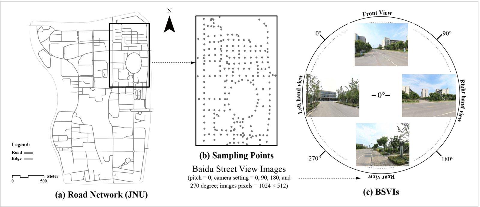
- Fix one sampling interval along the network and record it. Twenty to fifty metres suits urban work, and the interval must be identical across every unit you intend to compare.
- Render a fixed set of headings per point — four at 0°, 90°, 180° and 270° is the common research pattern — with field of view and pitch held constant for the whole project.
- Reproject panoramas to rectilinear crops before inference. Models are trained on ordinary photographs, and equirectangular input presents them with curved facades and stretched skies they have never seen.
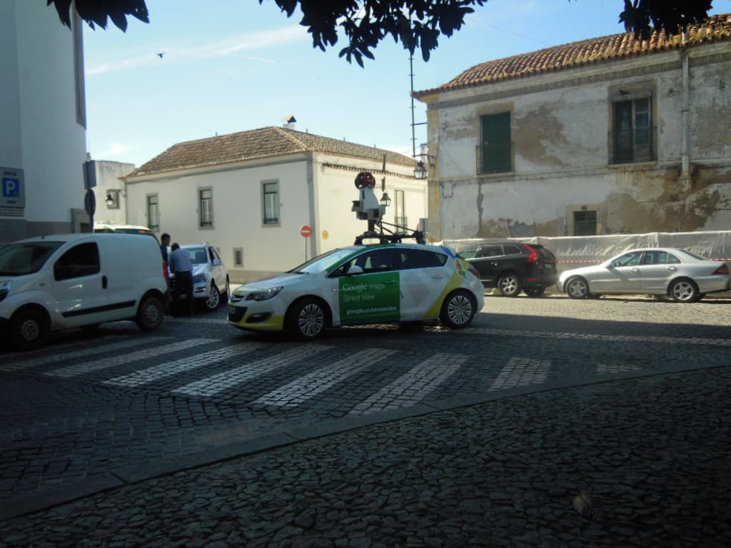
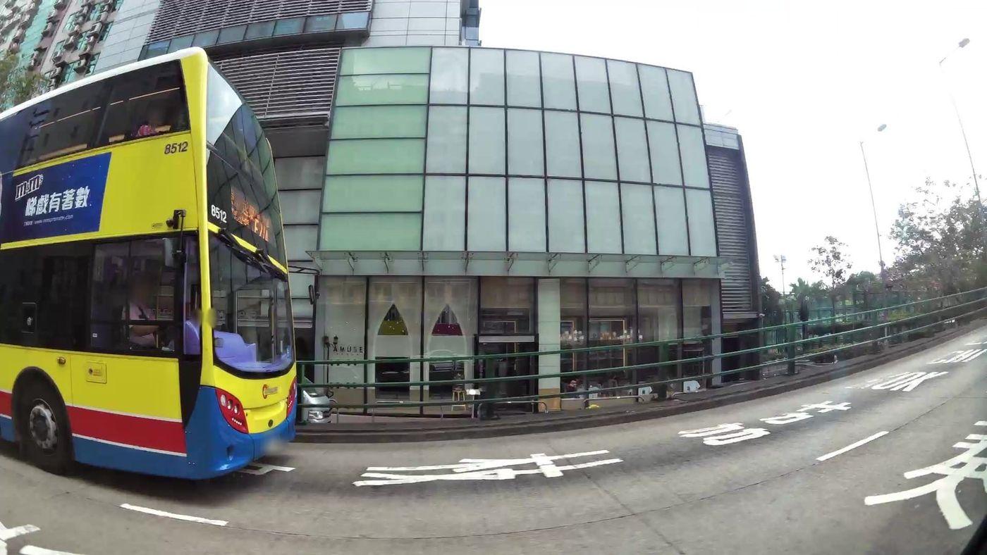
- Screen for the frames that quietly poison a batch: grey placeholders returned with a success status, indoor panoramas near a street point, a passing lorry filling the field of view, heavy lens flare, and rain on the lens.
- Write a manifest row per frame carrying source, licence, capture month and the exact camera parameters. Everything downstream is a claim about that specific field of view, and without the manifest the claim cannot be reconstructed.
Visual feature layer: four techniques, four kinds of evidence
- Semantic segmentation assigns a class to every pixel, which gives you proportions of the visual field: how much road, vegetation, sky or building a viewer at that point can see.
- Object detection returns discrete instances with boxes, which gives you counts and positions: signs, lamp posts, bins, parked cars, pedestrians.
- Text recognition reads the strings in the scene — shop fascias, street name plates, regulatory signs — turning imagery into something you can join to a business register.
- Learned embeddings compress a frame into a vector, which supports similarity search, clustering of streetscape types, and the regression heads used by perception models.
Choosing between them is not a matter of sophistication. A share and a count answer different questions: one pedestrian close to the lens can outweigh a dozen further away in pixel terms, so an activity indicator built from segmentation alone will disagree with one built from detection, and both can be right about their own definition.
Spatial indicator layer: point, segment, area
A per-frame number is not yet useful to a planner, because nobody makes decisions about a field of view. The aggregation runs in three steps: average the headings into one profile per sample point, join points to the street segment they belong to, then roll segments up to whatever unit the decision is made in. Each step needs a rule written down — how many points a segment needs before it gets a value, what happens to segments with one point, and whether points from different capture months may be averaged together at all.
Semantic segmentation is the workhorse
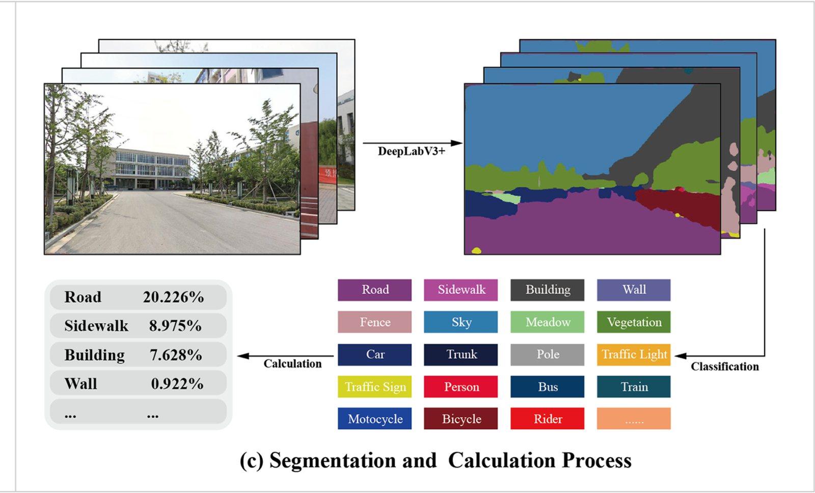
Most street view indicators in the literature come from one operation: classify every pixel, then count. The label space that dominates urban-scene work comes from Cityscapes, and its classes map directly onto the things urban research wants to measure.
| Class | What it supports |
|---|---|
| Road | Carriageway share, an approximation of how much of the scene is given to vehicles |
| Sidewalk | Pedestrian provision, and — with care — continuity along a corridor |
| Building | Vertical surface, the numerator of most enclosure proxies |
| Vegetation | Green view index, and seasonal comparison when the capture month is controlled |
| Sky | Openness, and the denominator of the enclosure proxy |
| Vehicle (car, truck, bus) | Traffic and parking presence at the moment of capture, and a major source of occlusion |
| Person and rider | Street activity at the moment of capture, always time-of-day dependent |
Green view index: what Treepedia actually measures
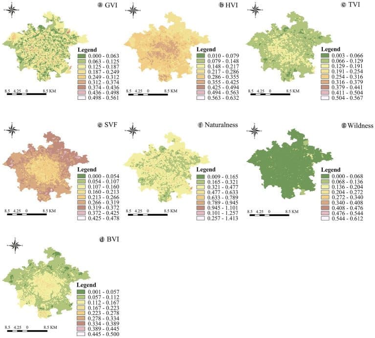
The green view index is the best-established street view indicator, and the clearest illustration of why the processing layer matters. It is the vegetation share of the visible frame, averaged across headings at a sample point — a measure of how much greenery a person standing on the pavement can see. The modified index published in Urban Forestry & Urban Greening in 2015 gave it a citable definition, and the Treepedia project at MIT Senseable City Lab applied the approach across many cities, which is how it became a comparable metric rather than a one-off method.
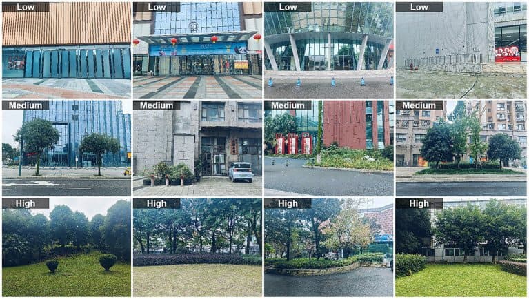
The same logic constrains the enclosure and openness family of indicators. A ratio of vertical surface to visible sky describes the perceived section of a street, not its measured section; building heights and street widths belong to cadastral and lidar data, and a project that needs the physical dimension should take it from there rather than infer it from pixels.
Urban perception: six attributes, and one large caveat
The second major application family predicts how people rate a place from its appearance. The approach that defined the field collected crowdsourced pairwise judgements — shown two street scenes, which looks safer? — at global scale, and trained models to predict the aggregated human preference. The Place Pulse 2.0 work built around six attributes: safe, beautiful, lively, wealthy, depressing and boring.
The pairwise design is the clever part. Asking someone to score a street from one to ten produces noise, because scales drift between raters; asking which of two streets looks safer produces a comparison that aggregates cleanly into a ranking. What the model then learns is the ranking, and the ranking is a statement about human judgement rather than about the street.
Walkability and accessibility
Traditional walkability audits send trained observers along streets with a checklist. Street-level imagery lets the same checklist be applied at a scale field audits cannot reach, and a body of work — including street-view-based walkability assessment published in the ISPRS International Journal of Geo-Information — has built indices on exactly that substitution.
- Sidewalk presence and continuity, detected per frame and then traced along a segment to find the breaks rather than the averages.
- Crossing facilities: marked crossings, signals, refuge islands, and where a desire line meets none of them.
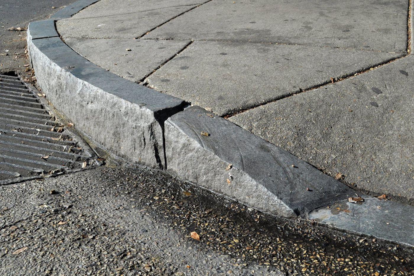
- Kerb ramps and steps at junctions, which is where an otherwise continuous route stops being usable by a wheelchair or a pushchair.
- Obstructions in the walking zone: poles, bins, parked vehicles, café spill-out, scaffolding.
- Buffering and comfort cues: street trees between pedestrian and traffic, lighting columns, seating.
Transport and road asset inventory
Asset work is the most operational application, and the one where detection rather than segmentation does the heavy lifting. The output is an inventory: a located, typed, deduplicated list of things on a corridor.
- Traffic signs and regulatory plates, typed by class and located along the segment.
- Street lighting: column positions and spacing, which feeds night-time coverage questions the imagery itself cannot answer.
- Lane markings and their apparent condition, plus crossing markings and stop lines.
- Pavement surface defects visible from the vehicle — cracking, patching, ponding — which suit triage rather than engineering assessment.
- Parking: on-street occupancy at the moment of capture, kerbside use, and loading activity.
Two constraints shape any asset job. Objects are detected once per frame but exist once in the world, so deduplication across overlapping frames is a real step and not an afterthought — an ordered capture sequence makes it far easier than a set of independent panoramas. And a single pass records one moment: a bin put out for collection, a van double-parked, a sign temporarily obscured by a delivery lorry. Inventory conclusions need either repeat passes or an explicit statement that they describe the capture instant.
Commerce and street life
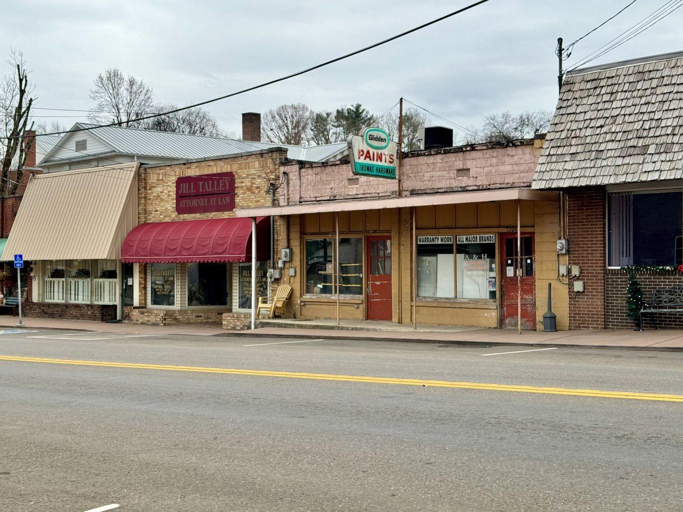
Retail and street-vitality work combines all three feature techniques. Text recognition reads shop fascias into names and, with a classifier, categories. Segmentation and detection describe the frontage itself — glazing against solid wall, shutters, awnings, spill-out — which is the physical interface between a building and the pavement. Detection counts the people and vehicles present.
- Sign OCR gives you a candidate business list per frontage, best used as a cross-check against a POI or business register rather than as a standalone census.
- Frontage transparency and shutter presence describe the quality of the ground-floor interface, which correlates with how a street is used but is not a measure of trade.
- Pedestrian and vehicle presence give an activity proxy for the frames you have, reported alongside the capture time.
Change detection over time
Repeat imagery at the same location is the most valuable and most easily botched application. When it works, it measures physical change directly: a lot developed, a frontage refurbished, a bike lane installed, trees planted or lost. Recent work on street-view time series for urban change assessment, including the CityPulse line of research, has built datasets and methods specifically for this, and the methodological care it takes is instructive.
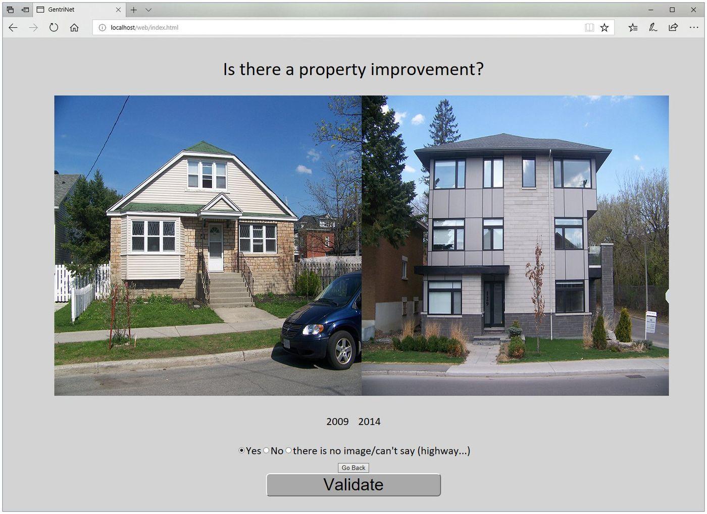
- Align the viewpoint. Panoramas from different years sit at slightly different positions along the street, so matching heading alone is not enough; render toward a fixed bearing and check the frames overlap on stable features such as building corners.
- Control season and illumination. Leaf-off against leaf-on will show a vegetation change that never happened, and a low-sun capture against an overcast one shifts every ground-class share.
- Hold the model and label schema fixed across all epochs, or the difference you measure includes a model upgrade.
- Separate real change from reprocessing. A new panorama identifier can mean new imagery or a re-render of the same capture, so confirm the capture date and returned location before calling anything a change.
- Validate the detected changes by eye on a sample. Change detection produces false positives at exactly the places that look most interesting — scaffolding, parked vehicles, temporary hoardings.
Health exposure and socio-economic proxies
Two application families extend street view indicators into other disciplines. In health research, eye-level greenery, enclosure and pedestrian provision are used as environmental exposure variables, on the reasoning that what a resident sees and walks through daily is closer to lived exposure than a district average from satellite data. In socio-economic work, streetscape features — building condition, vehicle types, frontage quality, greenery — are used to estimate income, deprivation or house prices in places where survey data is sparse or out of date.
Research design decides whether any of this holds
The applications above are only as good as the design underneath them, and the same handful of design fields explain most published disagreements. Treat these as required columns in the delivered table, not as method-section boilerplate.
- Sampling interval, identical across every unit you compare, and the snap radius that decided which panorama each point matched.
- Heading set, field of view and pitch, held constant project-wide. Widening the field of view alone will move every share you report.
- Capture month, carried through to the final table. Seasonality is systematic, not random, so it survives aggregation and turns into a finding.
- Source, where the imagery mixes platforms or includes your own capture. Different cameras and mounting heights shift indicators by more than many of the differences under study.
- Model identity, weights and label schema version, so a later re-run can be compared rather than merely repeated.
- Manual validation on a stratified sample, reported as an error distribution for this imagery, this model and this sample — not as a general accuracy claim.
- Point count per aggregation unit, alongside every aggregated value. A segment with one usable frame and a segment with twelve should not appear identical in the output.
Choosing a processing route
Most scoping conversations get faster once the question is stated precisely, because the route follows from it — and so does the honest list of what the route will not settle.
| What you are actually asking | Processing route | What it cannot settle |
|---|---|---|
| How much greenery can a pedestrian see here? | Segmentation → vegetation share per heading → green view index per segment, within one season window | Canopy area, species, or whether the greenery is publicly accessible |
| How enclosed does this street feel? | Segmentation → vertical surface against visible sky, with pitch and field of view fixed | Measured building heights or street widths; take those from cadastral or lidar data |
| How do people rate this street? | Perception model trained on rated pairs, revalidated on local raters before use | Whether the street is in fact safe, wealthy or lively |
| Is the pedestrian route continuous and usable? | Segmentation for sidewalk continuity plus detection of crossings, ramps and obstructions, traced along the segment | Compliance with an accessibility standard, which needs measured dimensions on site |
| What assets sit on this corridor? | Detection along an ordered capture sequence, deduplicated across overlapping frames | The condition of anything the camera could not see, and anything present only at other times |
| What businesses front this street? | Sign OCR plus frontage classification, reconciled against a POI or business register | Current occupancy, if the imagery is older than the local churn rate |
| What has changed here since an earlier year? | Aligned repeat imagery, same model and season window, with detected changes validated by eye | Anything at locations whose earlier captures you cannot actually obtain |
Reading the third column before starting is what separates a study that survives review from one that has to be re-scoped after the data is collected. It is also the cheapest part of the whole exercise.
Related services
- Street View Data Collection & ProcessingCoverage audit, sampling design, acquisition, QA and structured output for large study areas.
- Semantic SegmentationPixel-level classification with a versioned class mapping and validated output.
- GIS AnalysisIndicators joined to street geometry and aggregated to the unit your decision uses.
- Request a QuoteSend the area and the fields. You get a written scope and a fixed price first.